This page demonstrates solving the 2D heat conduction fin problem using a Gmsh-generated mesh. It is a
variation of the rectangular fin tutorial, but applied
to a rhomboidal domain.
Gmsh
![]() is a powerful mesh generation tool that can create complex geometries and meshes for finite element
analysis. For the mathematical formulation and theory, see the
basic tutorial.
is a powerful mesh generation tool that can create complex geometries and meshes for finite element
analysis. For the mathematical formulation and theory, see the
basic tutorial.
This example demonstrates how to import a Gmsh-generated mesh (.msh file format) and solve
a heat conduction problem.
<body>
  <!-- ...body region... -->
  <script type="module">
    // Import FEAScript library
    import { FEAScriptModel, importGmshMesh, plotInterpolatedSolution, printVersion } from "https://core.feascript.com/dist/feascript.esm.js";

    window.addEventListener("DOMContentLoaded", async () => {
      // Print FEAScript version in the console
      printVersion();

      // Fetch the mesh file
      const response = await fetch("./rhom_quad.msh"); // .msh version 4.1 is currently supported
      if (!response.ok) {
        throw new Error(`Failed to load mesh file: ${response.status} ${response.statusText}`);
      }
      const meshContent = await response.text();

      // Create a File object with the actual content
      const meshFile = new File([meshContent], "rhom_quad.msh");

      // Create and configure model
      const model = new FEAScriptModel();
      model.setModelConfig("heatConductionScript");

      // Parse the mesh file
      const rhom_quad = await importGmshMesh(meshFile);

      // Define mesh configuration with the parsed rhom_quad
      model.setMeshConfig({
        parsedMesh: rhom_quad,
        meshDimension: "2D",
        elementOrder: "quadratic",
      });

      // Apply boundary conditions using Gmsh physical group tags
      model.addBoundaryCondition("0", ["constantTemp", 200]); // Bottom boundary
      model.addBoundaryCondition("1", ["constantTemp", 200]); // Right boundary
      model.addBoundaryCondition("2", ["convection", 1, 20]); // Top boundary
      model.addBoundaryCondition("3", ["symmetry"]); // Left boundary

      // Solve
      model.setSolverMethod("lusolve");
      const result = model.solve();

      // Plot results
      plotInterpolatedSolution(model, result, "contour", "resultsCanvas");
    });
  </script>
  <!-- ... rest of body region... -->
</body>
For details on the Gmsh workflow, physical groups, and boundary condition mapping, please refer to the rectangular fin tutorial.
.geo File
Below is the rhom.geo file used in this tutorial. It defines a 4 m × 2 m rectangular domain
with physical lines for each boundary edge:
// 2D Rhomboid: 4m (base width) x 2m (height)

lc = 0.7; // Characteristic length

dx = 1.0; // Horizontal skew amount (controls rhomboid angle)

// Points (x, y, z, mesh size)
Point(1) = {0,    0, 0, lc}; // Bottom left
Point(2) = {4,    0, 0, lc}; // Bottom right
Point(3) = {4+dx, 2, 0, lc}; // Top right (shifted)
Point(4) = {dx,   2, 0, lc}; // Top left  (shifted)

// Lines
Line(1) = {1, 2}; // bottom
Line(2) = {2, 3}; // right
Line(3) = {3, 4}; // top
Line(4) = {4, 1}; // left

// Line Loop and Surface
Line Loop(1) = {1, 2, 3, 4};
Plane Surface(1) = {1};

// Physical Lines
Physical Line("bottom") = {1};
Physical Line("right")  = {2};
Physical Line("top")    = {3};
Physical Line("left")   = {4};

// Physical Surface
Physical Surface("domain") = {1};

// Generate 2D mesh
Recombine Surface{1}; // Turn triangle elements into quadrilaterals
Mesh.ElementOrder = 2; // Set quadratic elements
Mesh 2;
To generate a mesh file from this .geo script, you would run:
gmsh rhom.geo -2 in your terminal.
Below is a visualization of the quadrilateral mesh generated with Gmsh. The mesh consists of 24 elements.
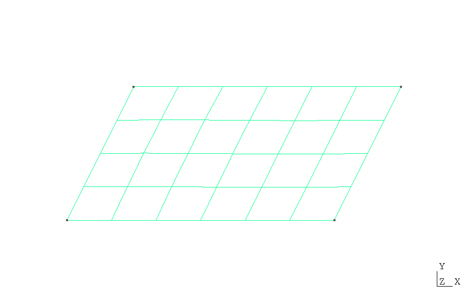
Quadrilateral mesh (rhom_quad.msh) generated using the
rhom.geo script with Gmsh
Below is the 2D contour plot of the computed temperature distribution. This plot is generated in real time using FEAScript.