
This page demonstrates solving the 2D heat conduction fin problem using a Gmsh-generated mesh.
Gmsh
![]() is a powerful mesh generation tool that can create complex geometries and meshes for finite element
analysis. For the mathematical formulation and theory, see the
basic tutorial.
is a powerful mesh generation tool that can create complex geometries and meshes for finite element
analysis. For the mathematical formulation and theory, see the
basic tutorial.
This example demonstrates how to import a Gmsh-generated mesh (.msh file format) and solve
a heat conduction problem.
<body>
  <!-- ...body region... -->
  <script type="module">
    // Import FEAScript library
    import { FEAScriptModel, importGmshQuadTri, plotSolution, printVersion } from "https://core.feascript.com/dist/feascript.esm.js";

    window.addEventListener("DOMContentLoaded", async () => {
      // Print FEAScript version in the console
      printVersion();

      // Fetch the mesh file
      const response = await fetch("./rect_quad_unstruct.msh"); // .msh version 4.1 is currently supported
      if (!response.ok) {
        throw new Error(`Failed to load mesh file: ${response.status} ${response.statusText}`);
      }
      const meshContent = await response.text();

      // Create a File object with the actual content
      const meshFile = new File([meshContent], "rect_quad_unstruct.msh");

      // Create and configure model
      const model = new FEAScriptModel();
      model.setSolverConfig("heatConductionScript");

      // Parse the mesh file first
      const result = await importGmshQuadTri(meshFile);

      // Define mesh configuration with the parsed result
      model.setMeshConfig({
        parsedMesh: result,
        meshDimension: "2D",
        elementOrder: "quadratic",
      });

      // Apply boundary conditions using Gmsh physical group tags
      model.addBoundaryCondition("0", ["constantTemp", 200]); // bottom boundary
      model.addBoundaryCondition("1", ["constantTemp", 200]); // right boundary
      model.addBoundaryCondition("2", ["convection", 1, 20]); // top boundary
      model.addBoundaryCondition("3", ["symmetry"]); // left boundary

      // Solve
      model.setSolverMethod("lusolve");
      const { solutionVector, nodesCoordinates } = model.solve();

      // Plot results
      plotSolution(
        solutionVector,
        nodesCoordinates,
        model.solverConfig,
        model.meshConfig.meshDimension,
        "contour",
        "resultsCanvas",
        "unstructured" // Important: specify unstructured mesh type for Gmsh meshes
      );
    });
  </script>
  <!-- ... rest of body region... -->
</body>
Important notes about the Gmsh workflow:
.geo file (see
Example Gmsh .geo File), you need to define physical groups
for boundaries using commands like Physical Line("bottom") = {1};. These are mapped to
tags in the imported mesh.
"1", "2", "3", "4", you
would reference them in FEAScript as "0", "1", "2",
"3", respectively. For example:
model.addBoundaryCondition("0", ["constantTemp", 200]); // Gmsh physical group tag 1.
This conversion is necessary because Gmsh uses 1-based indexing while FEAScript uses 0-based indexing.
"unstructured"
parameter to the plotSolution function to ensure correct visualization.
You can create your own Gmsh files by writing .geo scripts or using Gmsh's GUI. For this
example, we used a simple rectangular domain defined in a .geo file with specific physical
groups for each boundary.
.geo File
Below is the rect.geo file used in this tutorial. It defines a 4m × 2m rectangular domain
with physical lines for each boundary edge:
// 2D Rectangle: 4m (width) x 2m (height) with physical lines for boundary labeling

lc = 0.7; // Characteristic length (mesh density)

// Points (x, y, z, mesh size)
Point(1) = {0, 0, 0, lc};     // Bottom left
Point(2) = {4, 0, 0, lc};     // Bottom right
Point(3) = {4, 2, 0, lc};     // Top right
Point(4) = {0, 2, 0, lc};     // Top left

// Lines
Line(1) = {1, 2}; // bottom
Line(2) = {2, 3}; // right
Line(3) = {3, 4}; // top
Line(4) = {4, 1}; // left

// Line Loop and Surface
Line Loop(1) = {1, 2, 3, 4};
Plane Surface(1) = {1};

// Physical Lines
Physical Line("bottom") = {1};
Physical Line("right")  = {2};
Physical Line("top")    = {3};
Physical Line("left")   = {4};

// Physical Surface (optional, for FEM domains)
Physical Surface("domain") = {1};

// Generate 2D mesh
Recombine Surface{1}; // Turn triangle elements into quadrilaterals
Mesh.ElementOrder = 2; // Set quadratic elements
Mesh 2;
Note how the physical line tags in the .geo file correspond to the boundary conditions in
our FEAScript code:
Physical Line("bottom") = {1}; →
model.addBoundaryCondition("0", ["constantTemp", 200]);
Physical Line("right") = {2}; →
model.addBoundaryCondition("1", ["constantTemp", 200]);
Physical Line("top") = {3}; →
model.addBoundaryCondition("2", ["convection", 1, 20]);
Physical Line("left") = {4}; →
model.addBoundaryCondition("3", ["symmetry"]);
To generate a mesh file from this .geo script, you would run:
gmsh rect.geo -2 in your terminal, which creates a rect.msh file that can be
imported into FEAScript.
Below is a visualization of the quadrilateral mesh generated with Gmsh. Notice how Gmsh creates an unstructured mesh with irregular elements that could potentially adapt to complex domain features.
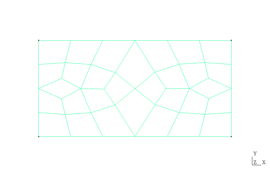
Quadrilateral mesh (rect_quad_unstruct.msh) generated using the
rect.geo script with Gmsh
The mesh consists of quadrilateral elements with varying sizes and shapes. This unstructured mesh approach would be particularly advantageous for complex geometries. FEAScript's Gmsh reader properly handles this unstructured mesh format and maps the elements and boundary conditions.
Below is the 2D contour plot of the computed temperature distribution. This plot is generated in real time using FEAScript. Please note that solutions computed on unstructured meshes like this may exhibit small numerical differences compared to solutions on structured orthogonal meshes. This occurs because derivative calculations in non-orthogonal elements are inherently less precise due to the Jacobian transformation process. These small differences are expected and acceptable for most engineering applications, but may be noticeable in regions with steep temperature gradients.