
In this tutorial, we address a stationary heat transfer problem within a two-dimensional rectangular domain. This is a typical cooling fin problem. Cooling fins are commonly used to increase the area available for heat transfer between metal walls and poorly conducting fluids such as air.
Steady heat conduction is described by the Laplace equation: \(\nabla^{2}T(x,y) = 0\), where \(T\) denotes the temperature.
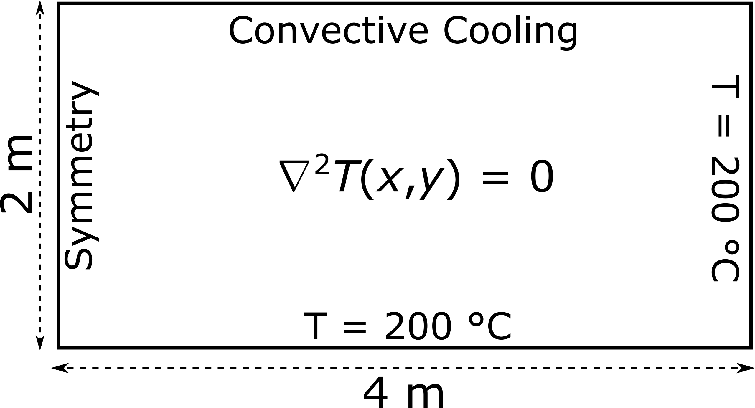
Schematic of the 2D cooling fin: constant temperature (200 °C) at bottom and right edges, symmetry (zero flux) at the left edge, and convection at the top edge (h/k = 1 m⁻¹, external temperature 20 °C)
The above schematic illustrates the problem domain and outlines the associated boundary conditions. The constant temperature boundary conditions are implemented as Dirichlet-type conditions in the finite element code. The symmetry boundary condition is implemented as a Neumann zero-flux type \( \left( \frac{dT}{dx}|_{x=0}=0 \right) \), while the convective cooling boundary condition is a Robin-type condition. Specifically, the latter is expressed as \(\frac{dT}{dy}|_{y=2}=-{\frac{h}{k}}(T-T_0)\), where \(h\) is the heat transfer coefficient, \(k\) the thermal conductivity and \(T_0\) is the external temperature. We assume here that \({\frac{h}{k}}\) = 1 m-1 and \(T_0\) = 20 °C.
Below is a demonstration of how to use the FEAScript library to solve this stationary heat transfer problem in your web browser. You only need a simple HTML page to run this example where the following code snippets should be included. First, load the required external libraries:
<head>
  <!-- ...head region... -->
  <script src="https://cdnjs.cloudflare.com/ajax/libs/mathjs/11.12.0/math.min.js"></script>
  <script src="https://cdnjs.cloudflare.com/ajax/libs/plotly.js/2.35.3/plotly.min.js"></script>
  <!-- ...rest of head region... -->
</head>
We should then define the problem parameters, such as the solver type, the geometry configuration, and the boundary conditions. This is performed using JavaScript objects directly in the HTML file:
<body>
  <!-- ...body region... -->
  <script type="module">
    // Import FEAScript library
    import { FEAScriptModel, plotSolution, printVersion } from "https://core.feascript.com/dist/feascript.esm.js";

    window.addEventListener("DOMContentLoaded", (event) => {
      // Print FEAScript version in the console
      printVersion();

      // Create and configure model
      const model = new FEAScriptModel();
      model.setSolverConfig("heatConductionScript");
      model.setMeshConfig({
        meshDimension: "2D",
        elementOrder: "quadratic",
        numElementsX: 8,
        numElementsY: 4,
        maxX: 4,
        maxY: 2,
      });

      // Apply boundary conditions
      model.addBoundaryCondition("0", ["constantTemp", 200]);
      model.addBoundaryCondition("1", ["symmetry"]);
      model.addBoundaryCondition("2", ["convection", 1, 20]);
      model.addBoundaryCondition("3", ["constantTemp", 200]);

      // Solve
      model.setSolverMethod("lusolve");
      const { solutionVector, nodesCoordinates } = model.solve();

      // Plot results
      plotSolution(
        solutionVector,
        nodesCoordinates,
        model.solverConfig,
        model.meshConfig.meshDimension,
        "contour",
        "resultsCanvas"
      );

    });
  </script>
  <!-- ...rest of body region... -->
</body>
In the boundary condition definition, the numbers at the left side (from "0" to
"3") indicate the boundaries of the geometry (the mesh generator of FEAScript has assigned
numbers to the boundaries, starting from the bottom boundary and proceeding clockwise). The
"constantTemp" condition sets a constant temperature value. The
"symmetry" boundary condition represents a zero-flux type. Finally, the
"convection" condition describes a convective heat transfer scenario. In addition, the
second argument of the "constantTemp" boundary condition corresponds to the constant
temperature value. For a "convection" boundary condition, the second argument represents
the \({\frac{h}{k}}\) value, and the third argument indicates the external temperature \(T_0\).
After solving the case, the results are shown in a 2D contour plot. To visualize it, include an HTML container where the plot will render:
<body>
  <!-- ...body region... -->
  <div id="resultsCanvas"></div>
  <!-- ...rest of body region... -->
</body>
The "resultsCanvas" is the id of the div where the plot will be rendered. This id is passed
as an argument to the plotSolution function to specify the target div for the plot.
Below is the 2D contour plot of the computed temperature distribution. This plot is generated in real time using FEAScript. You can find a Node.js implementation of this tutorial in the example directory.
See also here for a tutorial using FEAScript in a separate thread (web worker) for improved responsiveness and here for a tutorial using an unstructured mesh generated by Gmsh.