Overview
Creeping flow in a 2D lid-driven cavity, on a generated triangle mesh.
This page solves the 2D lid-driven cavity creeping flow problem on a mesh of triangles that
FEAScript generates itself, from the geometry of the domain, with
elements: "triangles". No mesh file and no external tool are needed. For the
formulation and the boundary conditions, see the
basic tutorial, which solves the same cavity
on a structured mesh of quadrilaterals.
The geometry is the same 4 × 2 rectangle as in the basic tutorial, and only the mesh settings
change, from quadrilaterals to triangles. A rectangle names its sides "bottom",
"right", "top" and "left", so the boundary conditions stay
the same:
<body>
  <!-- ...body region... -->
  <script type="module">
    import {
      FEAScriptModel,
      plotInterpolatedSolution,
      version,
    } from "https://core.feascript.com/dist/feascript.esm.js";

    window.addEventListener("DOMContentLoaded", () => {
      console.log("FEAScript version:", version);

      // 1. Create the model and select the physics
      const model = new FEAScriptModel();
      model.setModelConfig("creepingFlow", {
        solver: { method: "lusolve" },
        coefficientFunctions: {
          viscosity: 1, // μ
        },
      });

      // 2. Define the geometry and mesh it with quadratic triangles of side 0.5 at most
      model.setGeometry({ rectangle: [4, 2] }); // Boundaries "bottom", "right", "top", "left"
      model.setMeshConfig({ elements: "triangles", elementOrder: "quadratic", size: 0.5, minAngle: 30 });

      // 3. Apply the boundary conditions, keyed by the boundary names
      model.addBoundaryCondition("bottom", { type: "constantVelocity", u: 0, v: 0 }); // Bottom wall
      model.addBoundaryCondition("left", { type: "constantVelocity", u: 0, v: 0 });   // Left wall
      model.addBoundaryCondition("top", { type: "constantVelocity", u: 1, v: 0 });    // Moving lid
      model.addBoundaryCondition("right", { type: "constantVelocity", u: 0, v: 0 });  // Right wall

      // 4. Solve
      const result = model.solve();

      // 5. Plot the results
      plotInterpolatedSolution(model, result, "contour", "velocityMagnitudeCanvas");
      plotInterpolatedSolution(model, result, "contour", "uVelocityCanvas", { field: "u" });
      plotInterpolatedSolution(model, result, "contour", "vVelocityCanvas", { field: "v" });
    });
  </script>
  <!-- ...rest of body region... -->
</body>
Creeping flow needs elementOrder: "quadratic". On triangles, FEAScript uses the
Taylor-Hood P2-P1 pair: the velocity on 6-node quadratic triangles and the pressure on the 3
corner nodes, the triangle counterpart of the Q2-Q1 quadrilaterals of the basic tutorial.
plotInterpolatedSolution evaluates the quadratic shape functions inside each
triangle, so the plots show the curved contours of the P2 solution. For the other mesh settings
(size, minAngle, graded sizes and holes), see the
fin on a generated triangle mesh.
Below is the mesh that the settings above generate: 128 quadratic triangles with 281 nodes (with FEAScript 0.4.0), all with angles of at least 30 degrees. It has about as many nodes as the 12 × 6 quadrilaterals of the basic tutorial (325).
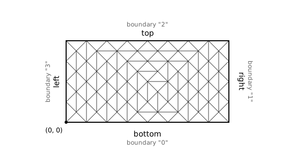
Quadratic triangle mesh of the 4 × 2 cavity, generated by FEAScript; the lid is the top side
Below are the 2D contour plots of the computed velocity magnitude \(|\mathbf{u}| = \sqrt{u^2+v^2}\), horizontal velocity component \(u\), and vertical velocity component \(v\), generated in real time with FEAScript. They match the quadrilateral results: the strongest return flow is \(u = -0.322\) here and \(-0.325\) on the quadrilaterals, a difference of 1%.
Velocity magnitude
Horizontal velocity (\(u\))
Vertical velocity (\(v\))
Stokes flow is mirror-symmetric about \(x = 2\), but this mesh is not, so the symmetry holds only up to the discretization error: at \((1, 1.5)\) and \((3, 1.5)\), \(u\) is 0.0755 and 0.0766. On the quadrilaterals, which are symmetric, the two values are equal. For a flow problem on a Gmsh mesh of quadratic triangles, see creeping flow through a 2D pillar array.
Stay in the loop
Join the mailing list.
Receive new tutorials, project updates and news.