Overview
Advection-Diffusion with a Gaussian Source Term Tutorial
In this tutorial, we address an advection-diffusion problem in a one-dimensional domain with a Gaussian source term. This is a fundamental transport phenomenon that occurs in many fields including fluid dynamics, heat transfer, and contaminant transport, where both diffusion and advection mechanisms are important.
The advection-diffusion equation is a partial differential equation that describes physical phenomena where particles, energy, or other physical quantities are transferred inside a physical system due to two processes: diffusion and advection. In one dimension, the steady-state equation is given by:
\(\frac{d^2u}{dx^2} - 10 \frac{du}{dx} = 10 \cdot e^{-200 \cdot (x - 0.5)^2}\)
This can be rewritten in the general form: \(\frac{d}{dx}\left(A(x)\frac{du}{dx}\right) + B(x)\frac{du}{dx} + C(x)u = D(x)\)
Where for our specific problem:
- \(A(x) = 1\) (diffusion coefficient)
- \(B(x) = -10\) (advection coefficient)
- \(C(x) = 0\) (no reaction term)
- \(D(x) = 10 \cdot e^{-200 \cdot (x - 0.5)^2}\) (Gaussian source term centered at x = 0.5)
We apply Dirichlet boundary condition at the left end: \(u(0) = 1\) and Neumann boundary condition (zero gradient) at the right end: \(\frac{du}{dx}(1) = 0\). These conditions represent a fixed concentration at the inlet and free outflow at the outlet of our domain. The Gaussian source term acts as a localized input at the center of the domain. The balance between diffusion (spreading) and advection (directed transport) will determine how the solution behaves.
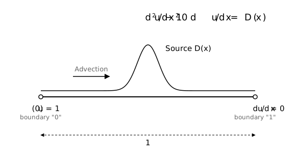
Schematic of the 1D domain: fixed value u(0) = 1 at the left end, zero gradient at the right end, and a Gaussian source centered at x = 0.5
Below is a demonstration of how to use the FEAScript library to solve this advection-diffusion problem in your web browser. You only need a simple HTML page to run this example where the following code snippets should be included. First, load the required external libraries:
<head>
  <!-- ...head region... -->
  <script src="https://cdnjs.cloudflare.com/ajax/libs/plotly.js/2.35.3/plotly.min.js"></script>
  <!-- ...rest of head region... -->
</head>
We should then define the problem parameters, such as the solver type, the geometry configuration, and the boundary conditions. This is performed using JavaScript objects directly in the HTML file:
<body>
  <!-- ...body region... -->
  <script type="module">
    import {
      FEAScriptModel,
      plotSolution,
      printVersion,
    } from "https://core.feascript.com/dist/feascript.esm.js";

    window.addEventListener("DOMContentLoaded", () => {
      console.log("FEAScript version:", printVersion);

      // 1. Create the model and select the physics: d²u/dx² - 10 du/dx = 10 exp(-200 (x - 0.5)²)
      const model = new FEAScriptModel();
      model.setModelConfig("generalFormPDEScript", {
        coefficientFunctions: {
          A: (x) => 1,                                          // Diffusion coefficient
          B: (x) => -10,                                        // Advection coefficient
          C: (x) => 0,                                          // Reaction coefficient
          D: (x) => 10 * Math.exp(-200 * Math.pow(x - 0.5, 2)), // Source term
        },
      });

      // 2. Define the mesh
      model.setMeshConfig({
        meshDimension: "1D",
        elementOrder: "quadratic",
        numElementsX: 20,
        maxX: 1.0,
      });

      // 3. Apply the boundary conditions
      model.addBoundaryCondition("0", ["constantValue", 1]); // Left
      model.addBoundaryCondition("1", ["zeroGradient"]);     // Right

      // 4. Solve
      model.setSolverMethod("lusolve");
      const result = model.solve();

      // 5. Plot the results
      plotSolution(model, result, "line", "resultsCanvas");
    });
  </script>
  <!-- ...rest of body region... -->
</body>
The mesh defined in step 2 divides the domain into 20 quadratic elements:
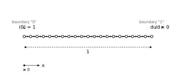
Mesh of the domain: 20 quadratic elements (41 nodes); open circles are the element end nodes, dots the midside nodes
After solving the case, the results appear as a line plot. To visualize it, include an HTML container where the plot will render:
<body>
  <!-- ...body region... -->
  <div id="resultsCanvas"></div>
  <!-- ...rest of body region... -->
</body>
The "resultsCanvas" is the id of the div where the plot will be rendered. This id
is passed as an argument to the plotSolution function to specify the target div for
the plot.
Below is the 1D line plot of the computed solution to the advection-diffusion equation. This plot is generated in real time using FEAScript. You can find a Node.js implementation of this tutorial in the example directory.
The solution shows the characteristic behavior of advection-diffusion problems. The magnitude and spread of the solution are determined by the balance between diffusion and advection.